Unlocking Efficiency: A Comprehensive Guide to Dynamic Programming

In the realm of computer science and algorithm design, efficiency reigns supreme. One powerful technique that enables developers to craft optimized solutions for complex problems is dynamic programming. This methodology, often perceived as daunting, is in reality a systematic approach to problem-solving that breaks down intricate challenges into smaller, overlapping subproblems. By solving each subproblem only once and storing its solution, dynamic programming avoids redundant computations, leading to significant performance gains. This article delves into the core concepts of dynamic programming, exploring its principles, applications, and practical implementation strategies. We’ll start with the fundamentals, progress through various examples, and conclude with insights into when and how to effectively leverage this technique.

Understanding the Fundamentals of Dynamic Programming

At its heart, dynamic programming is an algorithmic paradigm that embodies both recursion and memoization. It is primarily applicable to problems exhibiting two key properties: optimal substructure and overlapping subproblems. Let’s dissect each of these:

Optimal Substructure

A problem is said to possess optimal substructure if the optimal solution to the overall problem can be constructed from the optimal solutions to its subproblems. In simpler terms, if you know the best way to solve smaller parts of the problem, you can combine those solutions to find the best way to solve the entire problem. For instance, consider finding the shortest path between two cities. If the shortest path from city A to city B passes through city C, then the path from A to C and the path from C to B must also be the shortest paths between those respective cities. This property makes dynamic programming a viable approach.

Overlapping Subproblems

Overlapping subproblems occur when the recursive algorithm revisits the same subproblems multiple times. Naive recursive solutions can become exponentially inefficient due to this repeated computation. Dynamic programming addresses this inefficiency by solving each subproblem only once and storing the result in a table (or other data structure). When the same subproblem is encountered again, the stored solution is retrieved directly, avoiding redundant calculations. This memoization technique is crucial for achieving the performance benefits of dynamic programming.

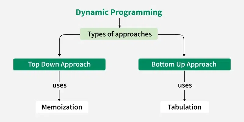
Approaches to Dynamic Programming: Top-Down vs. Bottom-Up

There are two primary approaches to implementing dynamic programming solutions: top-down (memoization) and bottom-up (tabulation).

Top-Down (Memoization)

The top-down approach starts with the original problem and recursively breaks it down into subproblems. Before solving a subproblem, the algorithm checks if the solution has already been computed and stored. If it has, the stored solution is returned directly. Otherwise, the subproblem is solved, the solution is stored, and then returned. This approach is often more intuitive and easier to implement, as it closely resembles the recursive formulation of the problem. However, it can incur some overhead due to the recursive function calls.

Example (Python):

def fibonacci_memoization(n, memo):
 if n in memo:
 return memo[n]
 if n <= 1:
 return n
 memo[n] = fibonacci_memoization(n-1, memo) + fibonacci_memoization(n-2, memo)
 return memo[n]

def fibonacci(n):
 memo = {}
 return fibonacci_memoization(n, memo)

print(fibonacci(10))

Bottom-Up (Tabulation)

The bottom-up approach starts with the smallest subproblems and iteratively builds up to the solution of the original problem. The solutions to the subproblems are stored in a table, and the algorithm fills in the table in a systematic order, ensuring that the solutions to all necessary subproblems are available when needed. This approach typically avoids the overhead of recursive function calls and can be more efficient in some cases. However, it may require more careful planning to determine the correct order in which to fill in the table.

Example (Python):

def fibonacci_tabulation(n):
 table = [0] * (n + 1)
 table[0] = 0
 if n > 0:
 table[1] = 1
 for i in range(2, n + 1):
 table[i] = table[i-1] + table[i-2]
 return table[n]

print(fibonacci_tabulation(10))

Applications of Dynamic Programming

Dynamic programming finds applications in a wide range of problem domains, including:

• Shortest Path Algorithms: Dijkstra’s algorithm and the Bellman-Ford algorithm can be viewed as instances of dynamic programming.
• Sequence Alignment: Used in bioinformatics to align DNA or protein sequences.
• Knapsack Problem: Determining the most valuable items to include in a knapsack with a limited weight capacity.
• Longest Common Subsequence: Finding the longest sequence that is a subsequence of two or more given sequences.
• Optimal Game Strategy: Determining the optimal moves for a player in a game.
• Compiler Design: Optimizing code generation and register allocation.

Illustrative Examples

Let’s explore a few examples to solidify our understanding of dynamic programming.

The Knapsack Problem

Imagine you have a knapsack with a limited weight capacity and a set of items, each with its own weight and value. The goal is to determine which items to include in the knapsack to maximize the total value without exceeding the weight capacity. This is a classic optimization problem that can be efficiently solved using dynamic programming.

The dynamic programming approach involves creating a table where rows represent items and columns represent weight capacities. Each cell in the table stores the maximum value that can be achieved with the items up to that row and the weight capacity up to that column. The table is filled in iteratively, considering whether to include each item or not, based on whether it increases the total value without exceeding the weight capacity.

Longest Common Subsequence (LCS)

Given two sequences, the longest common subsequence (LCS) is the longest sequence that is a subsequence of both sequences. For example, the LCS of “ABCBDAB” and “BDCABA” is “BCAB”.

The dynamic programming solution involves creating a table where rows represent the characters of the first sequence and columns represent the characters of the second sequence. Each cell in the table stores the length of the LCS of the prefixes of the two sequences up to that row and column. The table is filled in iteratively, comparing the characters at each position and updating the LCS length accordingly.

When to Use Dynamic Programming

While dynamic programming is a powerful tool, it’s not always the best solution. Here are some guidelines to help you determine when to use dynamic programming:

• Optimal Substructure: The problem must exhibit optimal substructure, meaning that the optimal solution to the overall problem can be constructed from the optimal solutions to its subproblems.
• Overlapping Subproblems: The problem must exhibit overlapping subproblems, meaning that the recursive algorithm revisits the same subproblems multiple times.
• Optimization Problem: Dynamic programming is typically used to solve optimization problems, where the goal is to find the best solution among a set of possible solutions.
• Polynomial Time Complexity: While dynamic programming can significantly improve performance compared to naive recursive solutions, it’s important to consider the time and space complexity of the dynamic programming solution. If the number of subproblems is too large, the dynamic programming solution may still be inefficient.

Advantages and Disadvantages

Advantages

• Efficiency: Dynamic programming can significantly improve the efficiency of algorithms by avoiding redundant computations.
• Optimality: Dynamic programming guarantees finding the optimal solution to the problem, provided that the problem exhibits optimal substructure.
• Systematic Approach: Dynamic programming provides a systematic approach to problem-solving, making it easier to design and implement algorithms.

Disadvantages

• Space Complexity: Dynamic programming often requires storing the solutions to subproblems in a table, which can consume a significant amount of memory.
• Complexity: Dynamic programming can be more complex to understand and implement than other algorithmic techniques.
• Applicability: Dynamic programming is not applicable to all problems. It is primarily suitable for problems exhibiting optimal substructure and overlapping subproblems.

Conclusion

Dynamic programming is a powerful algorithmic technique that can be used to solve a wide range of optimization problems efficiently. By breaking down complex problems into smaller, overlapping subproblems and storing the solutions to these subproblems, dynamic programming avoids redundant computations and guarantees finding the optimal solution. While it may require more careful planning and implementation than other algorithmic techniques, the performance benefits of dynamic programming can be significant. Understanding the principles of dynamic programming and its applications is essential for any computer scientist or software engineer seeking to develop efficient and optimized solutions.

Mastering dynamic programming requires practice and a solid understanding of its underlying principles. By working through various examples and applying the techniques discussed in this article, you can unlock the power of dynamic programming and become a more effective problem-solver. Remember to analyze the problem carefully, identify the optimal substructure and overlapping subproblems, and choose the appropriate approach (top-down or bottom-up) for implementation. With dedication and perseverance, you can conquer the challenges of dynamic programming and reap its rewards in terms of efficiency and optimality.

[See also: Related Article Titles]