Table of Contents

Q-Learning Example: A Practical Guide to Reinforcement Learning

Reinforcement learning, a subset of machine learning, empowers agents to learn optimal behaviors through trial and error. Among various reinforcement learning algorithms, Q-learning stands out for its simplicity and effectiveness. This article delves into a comprehensive Q-learning example, providing a practical understanding of its implementation and application. We’ll explore the core concepts, walk through a step-by-step implementation, and discuss real-world scenarios where Q-learning shines. This exploration aims to demystify Q-learning, making it accessible to both beginners and experienced practitioners.

Understanding the Fundamentals of Q-Learning

At its heart, Q-learning is an off-policy, temporal difference learning algorithm. Let’s break down this jargon:

Off-policy: The algorithm learns the optimal policy independent of the agent’s actions. This means it can learn from experiences generated by a different policy or even random exploration.
Temporal Difference (TD) Learning: TD learning updates estimates based on other estimates. In Q-learning, the algorithm updates the Q-value of a state-action pair based on the immediate reward and the estimated optimal future reward.

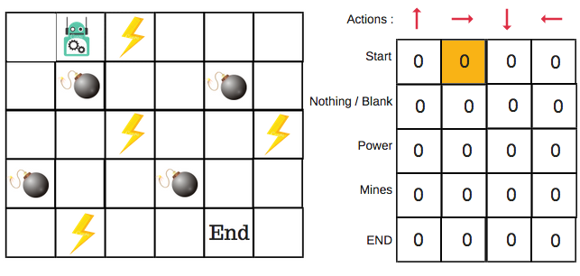
The core of Q-learning revolves around the Q-table (or Q-function). The Q-table is a matrix where rows represent states, columns represent actions, and each cell (Q-value) represents the expected cumulative reward for taking a specific action in a specific state. The goal of Q-learning is to learn the optimal Q-values, which represent the best possible action to take in each state.

The Q-Learning Equation

The Q-learning update rule is defined by the following equation:

Q(s, a) = Q(s, a) + α [R(s, a) + γ * maxₐ’ Q(s’, a’) – Q(s, a)]

Where:

Q(s, a) is the Q-value for state ‘s’ and action ‘a’.
α (alpha) is the learning rate (0 < α ≤ 1). It determines how much of the new information overrides the old information. A value of 0 means the agent learns nothing, while a value of 1 means the agent completely replaces the old value with the new one.
R(s, a) is the reward received after taking action ‘a’ in state ‘s’.
γ (gamma) is the discount factor (0 ≤ γ ≤ 1). It determines the importance of future rewards. A value of 0 means the agent only considers immediate rewards, while a value of 1 means the agent considers all future rewards equally.
s’ is the next state after taking action ‘a’ in state ‘s’.
a’ is the action that maximizes the Q-value in the next state s’.
maxₐ’ Q(s’, a’) is the maximum Q-value achievable from the next state s’.

A Step-by-Step Q-Learning Example: The FrozenLake Environment

To illustrate Q-learning in action, we’ll use the FrozenLake environment from OpenAI Gym. This environment represents a frozen lake where the agent’s goal is to navigate from the starting point (S) to the goal (G) without falling into any holes (H). The lake is represented as a grid of states.

Environment Setup

First, let’s install the necessary libraries:

pip install gym numpy

Then, import the libraries and create the FrozenLake environment:

import gym
import numpy as np

env = gym.make('FrozenLake-v1', is_slippery=False) # Setting is_slippery to False for deterministic behavior
state_space = env.observation_space.n
action_space = env.action_space.n

Here, `is_slippery=False` makes the environment deterministic, meaning the agent always moves in the intended direction. This simplifies the Q-learning example for demonstration purposes. If you want to make the environment harder, set it to `True`.

Initializing the Q-Table

Next, we initialize the Q-table with zeros:

q_table = np.zeros((state_space, action_space))

This creates a Q-table with `state_space` rows and `action_space` columns, all initialized to zero.

Q-Learning Algorithm Implementation

Now, let’s implement the Q-learning algorithm:

num_episodes = 1000
learning_rate = 0.9
discount_factor = 0.9

for episode in range(num_episodes):
    state = env.reset()
    done = False

    while not done:
        # Choose an action (Exploitation)
        action = np.argmax(q_table[state, :])

        # Take the action and observe the next state and reward
        new_state, reward, done, info = env.step(action)

        # Update the Q-table
        q_table[state, action] = q_table[state, action] + learning_rate * (reward + discount_factor * np.max(q_table[new_state, :]) - q_table[state, action])

        # Update the state
        state = new_state

print("Q-table:")
print(q_table)

In this code:

`num_episodes` determines the number of episodes the agent will learn from.
`learning_rate` and `discount_factor` are the parameters discussed earlier.
Inside the loop, the agent chooses an action based on the current Q-table (exploitation). In a real-world scenario, you would typically add an exploration component (e.g., epsilon-greedy) to balance exploration and exploitation.
The agent takes the chosen action and observes the next state and reward.
The Q-table is updated using the Q-learning equation.

Evaluating the Learned Policy

After training, we can evaluate the learned policy:

total_reward = 0
num_eval_episodes = 100

for episode in range(num_eval_episodes):
    state = env.reset()
    done = False
    episode_reward = 0

    while not done:
        action = np.argmax(q_table[state, :])
        new_state, reward, done, info = env.step(action)
        episode_reward += reward
        state = new_state

    total_reward += episode_reward

average_reward = total_reward / num_eval_episodes
print(f"Average reward over {num_eval_episodes} episodes: {average_reward}")

This code evaluates the agent’s performance over `num_eval_episodes` episodes and calculates the average reward. A higher average reward indicates a better-learned policy.

Addressing Exploration vs. Exploitation

The provided Q-learning example uses a purely exploitative approach after each episode. In practice, balancing exploration and exploitation is crucial for effective learning. A common technique is the epsilon-greedy strategy, where the agent chooses a random action with probability epsilon (exploration) and the best-known action with probability 1-epsilon (exploitation). Epsilon is often decreased over time to encourage more exploitation as the agent learns.

Real-World Applications of Q-Learning

Q-learning has found applications in various domains, including:

Robotics: Training robots to perform tasks such as navigation, object manipulation, and assembly.
Game Playing: Developing AI agents for games like chess, Go, and video games.
Resource Management: Optimizing resource allocation in areas like traffic control, energy management, and supply chain management.
Finance: Developing trading strategies and risk management systems.

Advantages and Disadvantages of Q-Learning

Advantages:

Simplicity: Q-learning is relatively easy to understand and implement.
Model-Free: It doesn’t require a model of the environment.
Off-Policy: It can learn from experiences generated by any policy.

Disadvantages:

Curse of Dimensionality: The Q-table can become very large for environments with a large state or action space.
Slow Convergence: Q-learning can be slow to converge, especially in complex environments.
Discrete Action Space: It’s typically used with discrete action spaces.

Conclusion

This Q-learning example provides a practical introduction to reinforcement learning. By understanding the fundamentals, implementing the algorithm, and exploring real-world applications, you can leverage Q-learning to solve complex problems in various domains. While Q-learning has its limitations, its simplicity and effectiveness make it a valuable tool in the arsenal of any machine learning practitioner. Remember to explore techniques like epsilon-greedy for balancing exploration and exploitation, and consider alternative reinforcement learning algorithms for environments with continuous action spaces or very large state spaces. [See also: Deep Reinforcement Learning Explained] As you delve deeper into the world of reinforcement learning, you’ll discover the power of algorithms like Q-learning in enabling agents to learn and adapt to complex environments. The journey of mastering Q-learning begins with understanding its core mechanics and experimenting with diverse applications. Continued practice and exploration will solidify your understanding and unlock the full potential of this powerful algorithm.